

Introduction
In today’s digital landscape, network security is a critical concern for businesses and organizations of all sizes. One of the tools used by security professionals to monitor and protect computer networks is Suricata, a powerful intrusion detection and prevention system. Suricata is open-source software that is used to monitor network traffic and alert security teams to potential threats.
MITRE ATT&CK is a globally accessible knowledge base of adversary tactics and techniques based on real-world observations. The framework provides a standardized vocabulary and methodology for describing and categorizing cyber threat tactics and techniques, which enables security teams to identify and respond to threats more effectively. Thus, mapping Suricata rules to MITRE ATT&CK tactics and techniques is important for identifying and responding to cyber threats effectively.
Given that there are tens of thousands of Suricata rules, manual mapping can be challenging due to several reasons. First, there are many Suricata rules, this complexity can make it challenging to identify the correct mapping. Second, the mapping process requires significant domain knowledge and expertise in network security, which may not be available to all security teams. Third, manual mapping is a tedious and repetitive task that can lead to errors due to human factors such as fatigue and distraction.
Automating the mapping process using machine learning algorithms can help overcome these challenges. Machine learning algorithms can be trained to recognize patterns in the data and make accurate predictions about the appropriate mapping of Suricata rules to MITRE ATT&CK tactics and techniques. However, developing an effective machine learning algorithm requires careful consideration of several factors, including the training data used, the algorithm used, and the evaluation metrics used to assess performance.
Methodology
Dataset
To train the model, we used the ET Open ruleset, which includes any signature contributed by the community or written by Proofpoint based on community research. This dataset was chosen due to its wide availability. As of 03 February 2023, the ET Open ruleset contained a total of 32,806 signatures.
However, only 2,878 signatures were mapped to MITRE ATT&CK tactics and techniques. These mapped signatures represent 11 MITRE techniques and were used as the labeled data for training the algorithm. The remaining signatures were not used in the training process.
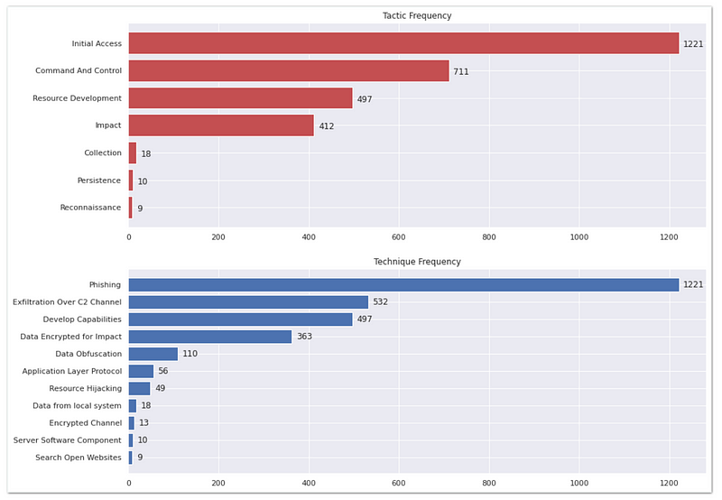
One of the challenges encountered in using this data was data imbalance. The data was heavily skewed, with the top two techniques already contributing to most of the data, 60% (1753 out of 2878). Additionally, some of the techniques have significantly lower data points than others. In fact, the bottom two techniques, Server Software Component and Search Open Websites, have only 10 (0.34%) and 9 (0.31%) data points respectively. This means that the algorithm would be more likely to predict these top techniques, while less frequently predicting the less common techniques.
Feature Selection
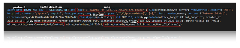
The following are the selected features utilized for training the model.
- The protocol component specifies the type of network protocol used in network traffic such as TCP, UDP, ICMP or IP. There are also a few application layer protocols such as HTTP, FTP and TLS.
- The traffic direction component specifies the direction of the network traffic, such as incoming (to HOME_NET) or outgoing (to EXTERNAL_NET). This information can help determine if the traffic originates from the attacker or the victim and can help identify the source or target of the attack.
- The msg feature contains a brief description of the network traffic that triggered the rule.
- The classtype keyword gives information about the classification of rules and alerts
- The tag feature is a user-defined field that can be used to categorize rules according to specific criteria.
There were some samples where the tag was either empty or had multiple tags. To avoid deleting the samples with empty tags (we did not want to further reduce our already limited dataset), we decided to choose a machine learning algorithm that could handle missing values. The output of the model is the corresponding MITRE ATT&CK tactic and technique that the network threat belongs to.
Given the existence of labelled signatures in the ET Open ruleset, we chose to adopt a supervised learning approach for this task. Several classification algorithms were evaluated including Naive Bayes, Random Forest, Logistic Regression, and Support Vector Machines (SVM).
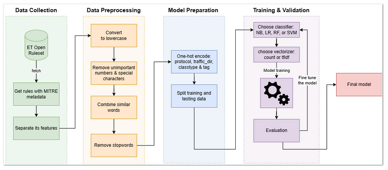
Data Preprocessing
Data preprocessing is the process of transforming raw data into a format that can be easily used by a machine learning algorithm. The purpose of data preprocessing is to prepare high-quality data that can be used to train a machine learning model effectively, by removing noise and inconsistencies and transforming the data into a format that can be easily understood by the algorithm.
In our data preprocessing methodology, we performed several rudimentary steps. These steps included converting all text to lowercase, removing unimportant numbers, removing special characters such as parentheses, brackets, slashes, and hyphens, and combining words that had the same meaning, such as ‘C2’ and ‘CNC’. We also removed stop words, which are common words that do not carry significant meaning in the context of our classification problem. It’s important to note that more complicated preprocessing techniques can always be employed to further enhance the results.
Model Training
After the data preprocessing is completed, the data is split into two sets, the training set, and the testing set. The training set, which constitutes 80% of the data, is used to train the models, while the remaining 20% is used to evaluate the performance of the models. The split is stratified based on each technique, ensuring that the distribution of classes in the training and testing sets are similar.
Regarding feature selection, for the ‘msg’ feature, we considered two feature extraction methods: CountVectorizer and TfidfVectorizer. CountVectorizer counts the frequency of each word in a document and creates a matrix of word counts. TfidfVectorizer stands for Term Frequency-Inverse Document Frequency Vectorizer, which also counts the frequency of each word in a document, but also takes into account how frequently the word appears in the entire corpus. It then assigns a score to each word that reflects its relevance to the document, with higher scores given to words that are more unique to the document.
To ensure the optimal feature extraction for this scenario, we decided to evaluate the performance of both CountVectorizer and TfidfVectorizer for each classifier model. Additionally, we chose to use one-hot encoding for the other features (protocol, traffic direction, classtype & tag) since it can be applied to categorical variables without any inherent order or ranking.
Model Evaluation Metrics
Performance evaluation is an essential step in assessing the effectiveness of the model. While accuracy is the most commonly used performance metric, it is not the preferred measure for classifiers, especially when dealing with skewed datasets. Suppose we have a classifier that can only guess the top 4 out 11 techniques correctly. If we evaluate the performance of this classifier using accuracy, we will get a score of: ((1221+711+497+363)/2878) * 100 = 97.01%. This might seem like a great score at first glance, but it is actually misleading. The reason is that the dataset is heavily skewed towards those top few categories, which has a much higher number of instances compared to the other categories. Thus, while it would achieve a high accuracy score, it would not be useful in practice.
In such cases, a much better way to evaluate the performance of a classifier is to look at the confusion matrix, which provides detailed information about the model’s performance in terms of true positives, false positives, true negatives, and false negatives.
Moreover, other metrics such as precision, recall, and F1-score are often used to evaluate the performance of classifiers. Precision measures the proportion of true positives among all the instances that the classifier labeled as positive. Recall, on the other hand, measures the proportion of true positives that the classifier correctly identified. Finally, F1-score is the harmonic mean of precision and recall, which provides an overall measure of the classifier’s performance.
The F1-score is designed to give equal importance to precision and recall by combining them into a single metric. It requires both precision and recalls having high values for the F1-score to increase. F1-score can be computed using different methods such as F1-micro and F1-macro. F1-micro computes the F1-score globally by counting the total true positives, false negatives, and false positives, while F1-macro computes the F1-score independently for each class and then averages the scores across all classes. So, if you care about each sample equally much, it is recommended to use the “micro” average f1-score; if you care about each class equally much, it is recommended to use the “macro” average f1-score
Results and Analysis
Comparison of Model Performance
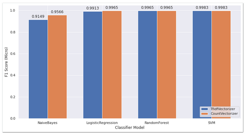
From the chart, it is evident that the CountVectorizer generally yields better performance for all models for F1-Micro. TfidfVectorizer shows comparable results for the Random Forest and SVM models. The SVM model has the best performance out of all models by achieving a score of 0.9983 for both feature extraction methods. Additionally, the performance of each model, after Naive Bayes, is significantly small, indicating that the performance of the models is largely dependent on the quality of the input features.
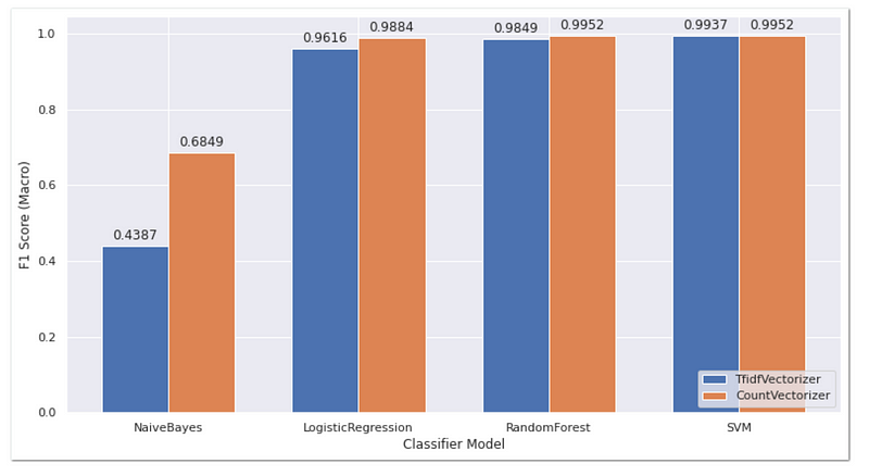
For F1-macro, the chart follows the same trend as the F1-micro scores, with CountVectorizer outperforming TfidfVectorizer. Similarly, SVM has the highest score out of all models for both feature selection methods. SVM with CountVectorizer achieves the highest score with 0.9952, making it the ideal classifier and feature selection to use as a model.
Classification Results in Confusion Matrix
The confusion matrix below provides a visual representation of both accurate and inaccurate predictions by the chosen model.
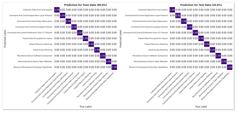
The left one shows the performance of the model on the training data, and the right one shows the performance on the test data. Overall, the model seems to be able to correctly predict all data that it has seen during the training phase, as evidenced by the high diagonal values in the left part of the matrix. However, the model’s performance on the test data is also high, but not perfect.
Looking at the confusion matrix for the test data, we can see that the model performs exceptionally well in predicting most of the classes. However, it seems that the model still struggles a bit to correctly distinguish between the two techniques of ‘Application Layer Protocol’ and ‘Exfiltration Over C2 Channel’. This suggests that further refinement of the features and additional training data may help improve the model’s performance in distinguishing between these classes.
Limitations and Future Work
There are several limits of these findings that need to be mentioned. First, the dataset used in this study is relatively small, and some of the samples are incredibly small, which is not optimal for testing, thus limiting the generalizability of the results. To address this limitation, future studies could explore using a larger dataset, such as combining ET Open ruleset with ETPRO ruleset.
Second, the preprocessing steps used are quite crude and need improvement. It is worth noting that the quality of the data is arguably the most important thing in training machine learning models. As the phrase goes, “garbage in, garbage out.” Thus, future studies should consider more sophisticated preprocessing techniques to ensure that the data is of high quality and suitable for training machine learning models.
Third, more (powerful) algorithms could be used and tested. While the models used in this study performed reasonably well, there may be other algorithms that could achieve even higher levels of accuracy. Future studies could explore these alternatives to identify the most effective algorithms for this task.
Fourth, other, more suitable features may be considered as input. It is possible that some relevant features were not included in this study and that other features may be more effective for this task. Therefore, future studies should explore alternative feature sets to determine which features are most useful for detecting network security threats. Overall, the limitations and future work of this study highlight the need for continued research in this area to improve the accuracy and effectiveness of machine learning-based network security threat detection.
Finally, incorporating human expertise and feedback may be beneficial to help the model learn from and adapt to new types of attacks. The model’s performance may also be impacted by changes in the threat landscape, so ongoing monitoring and updates may be necessary to maintain its effectiveness. Overall, the machine learning model shows promise for mapping Suricata rules to MITRE ATT&CK, but continued development and testing are necessary to fully evaluate its potential.
Conclusion
In conclusion, these findings highlight the importance of using machine learning and frameworks like MITRE ATT&CK to improve the detection and classification of cybersecurity threats. We hope that these findings provide valuable insights and benefits for the information security community. By mapping the Suricata rules to MITRE ATT&CK tactics and techniques, security analysts can gain a better understanding of the attacks they are facing and take proactive steps to protect their organizations. The use of machine learning algorithms can further enhance detection capabilities and provide more accurate and reliable threat intelligence.